JASP Tutorial Center

Table of Contents

Introduction

Descriptive Analyses

Independent Samples T-Test

Paired Samples T-Test

One Sample T-Test

ANOVA
Linear Regression

Introduction

JASP is a user-friendly statistical software designed to make data analysis accessible to researchers & students. Having strong JASP skills is crucial for PSYC 2260, PSYC 3630, PSYC 3340, PSYC-4520 and any projects involving statistics/data analysis.

To download the JASP program for free, please visit https://jasp-stats.org/

Descriptive Analyses

A pattern you will notice often here is an assumption in each topic. In this case, it is assumed that you have some knowledge of the scales of measurement and basic statistics. If you do not know about such concepts, it may be difficult to understand descriptive analyses.

To get started, we will be working with a hypothetical data set (Table 1). The data set contains 14 participants, randomized into two groups, a control & an experimental group. Participants in the control group sit in a white, blank room with a chair for 5 minutes, and participants in the experimental group sit in a room with a chair, but the room is filled with vegetation, has artificial sunlight and nature sounds -- attempts to simulate a "jungle-like" setting as much as possible.

To download the dataset, please click here.

Both groups would fill out a Perceived Stress Scale (PSS) form, whereas stress is measured on a scale of 0 to 40. Scoring 0 represents the participant is incredibly stressed and perceives the situation as stressful, and 40 represents no apparent stress.

We are interested in figuring out the mean, median, and Std. deviation for both groups. With JASP open, the steps are as follows:

Assumptions: Basic stats (means, std. deviation, median) & scales of measurement.

Table 1. Hypothetical data for control & experimental groups

1. Import the data: go to ≡ and click "Open" - then select the .csv file

2. Set both variables as "Scale" - as shown in the video.

3. Click "Descriptives"

4. Drag your two variables "Control" and "Experimental" into the "Variables" box.

5. On the statistics tab, enable Mean, Median, Mode, Std. deviation.

Upon successful completion of these steps, you should have your basic descriptive analyses for both groups. You can also experiment around with the software and enable some plots, such as distribution & Q-Q plots.

Tutorial video for descriptive analyses. Different values are used than the data presented here.

Knowledge Assessment

Now it's your turn to run the statistical analyses on the PSS data set provided on the website. Please note that the numbers displayed in the video are different than your data. Error margin for answers: +/- 0.01

Independent Samples T-test aka Standard T-Test

It is important to remember that statistical tests are always a test on your null hypothesis. In other words, it determines the probability that your null hypothesis is valid.

An independent samples t-test is a fundamental type of statistical test applied ONLY when you need to compare the means of precisely TWO groups (no more, no less), such as the Control Group vs the Experimental Group.

Please proceed by revising your data such that all the participants have the stress variable and are assigned a grouping variable. In this case, 0 represents the control group, and 1 represents the experimental group (Table 2). Implementing these changes makes it easier for JASP to analyze your data, and organizing the data with a grouping variable is good data practice. Let's first apply labels to our variables before running the independent samples t-test.

Assumptions: t-distribution, z-score, hypothesis testing

1. Import the data: go to ≡ and click "Open" - then select the .csv file

2. Set the stress variable as "Scale"

3. Set the group variable as "Nominal"

4. Apply labels by clicking on the group variable and applying a label of control for 0 and experimental for 1 - as shown in video

Upon successful completion of these steps, you should have an independent samples-test table containing various rows that provide statistical information: t, df, p, etc. You should also have your effect size & confidence intervals listed on the table, and your descriptives table & descriptive graphs.

By selecting Group ≠ Group 2, you are conducting a two-tailed test.

Tutorial video for applying group labels.

Table 2. Revised hypothetical data.

Then, let's proceed with running the t-test:

1. Click T-Tests, in which a dropdown menu will appear.

2. In that menu, click independent samples t-test.

3. Drag Stress into the "Variables" box.

4. Drag Group into the "Grouping Variable" box.

5. Enable "Location parameter" & "confidence interval" at (95%).

6. In Tests, enable Student.

7. In Effect Size, enable "Cohen's d"

8. For this data set, enable Group 1 ≠ Group 2 hypothesis.

9. Enable Descriptives and Descriptives Plots

10. Optional: In Assumption Checks, enable Normality.

Tutorial video for running an independent samples t-test.

Independent Samples T-test output

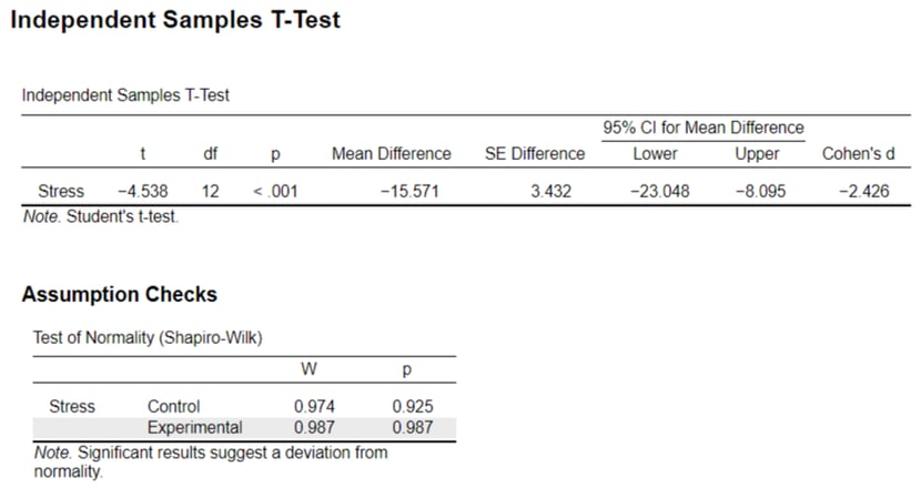
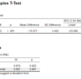
Your t-test results will provide you with the following information to determine whether your null hypothesis needs to be accepted or rejected. Let's briefly look over the key units/concepts in this output:

1. t-value (t): Measures how sample mean differs from population mean in standard error units, used in hypothesis testing for group differences.

2. Degrees of Freedom (df): Values free to vary in a calculation, used in t-tests to determine critical values.

3. p-value (p): Probability of obtaining a test statistic as extreme as observed, assuming null hypothesis is true. Conventionally, p < 0.05 indicates significance and the null hypothesis should be rejected.

4. Mean Difference: Numerical gap between group averages, quantifies effect size.

5. SE Difference: Measures variability in estimated difference between sample means, indicates precision.

6. Cohen's d: Standardized effect size, quantifies group difference in standard deviation units, useful for assessing the magnitude of mean differences.

You will see in this example we ran an assumption check, specifically a Test of Normality (Shapiro-Wilk), which determines whether the data for each of the groups is normally distributed. If the results are significant (W), it indicates that the data is not normally distributed, and another statistical method is recommended for analyzing the data. It is ALWAYS important to run assumptions in your data, but this is a concept not often taught in 2nd year psychology. You may have noticed a homogeneity of variance assumption check box when running a t-test -- this is also a very important assumption as many tests rely on the assumption of equal variances in different groups.

Knowledge Assessment

Now, it is time to interpret the results of these statistics findings. It is important to interpret these results carefully and what they mean for the data at hand. It is also recommended to run the analysis yourself as it serves as good statistics & data analysis experience.

Paired Samples T-test

The paired samples t-test is another method for detecting differences (and highly sensitive) in your data. It is primarily used in Before vs. After experiments, where the same participants are measured in a before condition and an after condition. In this case, we are going to modify our data and its format. It will contain 7 participants, and they will have their stress evaluated before the treatment is implemented (the nature room), and then it will be measured after they undergo treatment (independent variable), refer to Table 3. To run the paired samples t-test, the instructions are as follows:

Assumptions: t-distribution, z-score, hypothesis testing

1. Import the data: go to ≡ and click "Open" - then select the .csv file

2. Set both variables as "Scale"

3. Click "T-Tests"

4. Select "Paired-Samples T-Test"

5. Drag your variables (variable pairs) into the Variable pairs box.

6. Enable Student, Location parameter, confidence interval of 95%

7. Enable Effect Size.

8. Enable Descriptives and Descriptives plots.

If done correctly, you should be able to see a statistical table similar to that of the independent samples T-test. In general, the null hypothesis structure for the paired t-test (two-tailed) is:

Hₒ: μ1 ≠ μ2

Table 3. Stress values in before vs. after conditions.

Tutorial video for running a paired samples t-test.

Knowledge Assessment

Let's employ the paired samples t-test and analyze the statistical outcomes. This should be familiar if you already have a solid grasp of hypothesis testing. The questions are in reference to the data presented in Table 3.

One Sample T-Test

In brief, a one-sample t-test essentially compares a SINGLE sample/group mean to a hypothesized population mean. For example, if you implemented a treatment that improved anxiety scores for participants, it can be compared to a well-established population mean (that is representative of your participants) and see whether the participants scored better or worse in comparison to that mean. To run the test, the instructions are as follows:

Assumptions: t-distribution, z-score, hypothesis testing

1. Import the data: go to ≡ and click "Open" - then select the .csv file

2. Set both variables as "Scale"

3. Click "T-Tests"

4. Select "One Sample T-Test"

5. Drag your variables (variable pairs) into the Variable pairs box.

6. Enable Student, Location parameter, confidence interval of 95%

7. Define your hypothesized value (Test value)

8. Enable Effect Size.

9. Enable Descriptives and Descriptives plots.

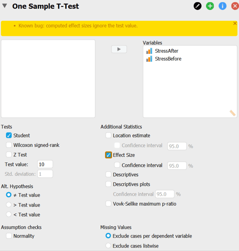
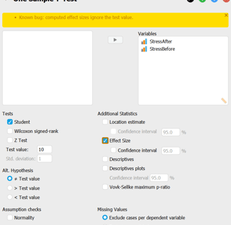
Fig 1. One Sample T-Test menu. The hypothesized value is 10 (test value).

ANOVA

ANOVA stands for "analysis of variance" which is important for comparing the means when you have more than 2 groups. It is important to understand the kinds of ANOVAs.

One-Way ANOVA: This test is used when comparing the means of THREE or MORE groups, which, unlike the t-tests, are limited to comparisons between two groups. Repeatedly using t-tests for multiple group comparisons in a single study is generally inappropriate due to statistical concerns.

Two-way ANOVA: This test is used to compare the means of TWO or MORE groups in response to TWO different independent variables. This is often vital for assessing the interaction effects between treatments.

So how do we run such an ANOVA? Well, it's simple.

1. Import the data: go to ≡ and click "Open" - then select the .csv file

2. Click "ANOVA"

3. Select "ANOVA" in the Classical Section

4. Drag your dependent variable onto the Dependent Variable box.

5. Drag your independent variable (such as treatment groups) to Fixed Factors.

6. If you have another independent variable (such as treatment dose), drag it into Fixed Factors, making this a two-way ANOVA.

Table 4. Sample two-way ANOVA data.
IV #1: Treatment group. 0 = Drug one, 1 = Drug two, 2 = Drug three.

IV #2: Dose. 0 = Small dose, 1 = Medium dose, 2 = Large dose.

Linear Regression

Linear regression is a very useful statistical test and is commonly used. Linear regression is to be utilized when you are comparing the means of groups along a continuum of THREE or MORE treatment levels. In other words, linear regression is powerful for examining continuous relationships, and you typically use it when you want to predict the value of a dependent variable based on one or more independent variables, where at least one of them is continuous.

Additionally, you can use it to analyze the means of responses across three or more treatment levels, whether these are spaced at consistent intervals, or like increasing dose levels by units of 5. A key outcome of this analysis is the "Best Fit" line that attempts to minimize the distance to all observed data points.

1. Import the data: go to ≡ and click "Open" - then select the .csv file

2. Click "Regression"

3. Select "Linear Regression" in the Classical Section

4. Drag your dependent variable onto the Dependent Variable box.

5. Drag your predictor variables into the Covariates box.

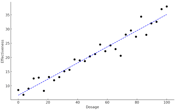
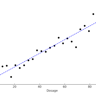
Fig 2. An example figure of a linear regression with a best fit line.

References

JASP Team. (2023). JASP (Version 0.18.1) [Computer software]. https://jasp-stats.org/